· rreck · ai · 5 min read
Quickly and safely using information from my Doctor's Office
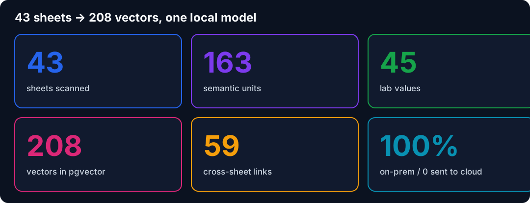
Forty-three scanned medical sheets, understood by a 3-billion-parameter model running on an on-premise 4080 GPU, turned into 208 searchable vectors and 45 tracked lab values — in eleven minutes, with nothing sent to the cloud. The pipeline, the timings, and the numbers.
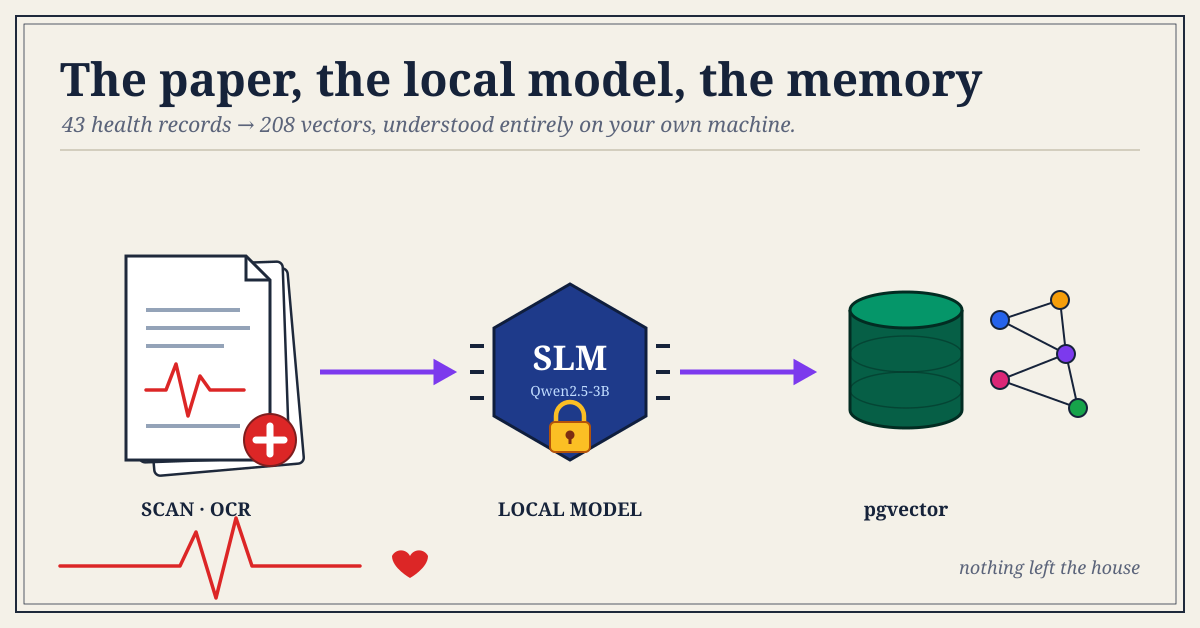
When you request your records from a doctor’s office, what arrives is a stack of paper: chart printouts, faxed laboratory reports, and letterhead correspondence. In that form a health history cannot be searched, and trends cannot be read across it; scanning it to PDF only exchanges a paper stack for a digital one. This post documents an end-to-end run that took forty-three sheets obtained from my GP’s office and turned them into a queryable semantic memory — with one hard constraint: every act of understanding is performed by a small language model running locally on my own hardware. Nothing in these documents was ever sent to a cloud model. Every figure below is read from the running system, snapshot 2026-07-11.
The workflow
A duplex document scanner feeds an OCR stage, whose text is handed to a local SLM for classification and semantic extraction. The extracted facts are embedded and stored in Postgres/pgvector, where cross-document similarity surfaces links no reader of the loose pages could see.

Mermaid source for this diagram
%%{init: {'flowchart': {'curve': 'basis'}}}%%
flowchart TD
    A([43 sheets · ScanSnap iX1500 ADF]):::scan -->|1.71s/sheet| B[TIFF per sheet]:::scan
    B -->|tesseract · 1.63s/sheet| C[OCR text + confidence]:::ocr
    C -->|prompt| D{{LOCAL SLM · Qwen2.5-3B · 4-way · 5.4s/sheet}}:::slm
    D -->|classify + extract| E[163 semantic units]:::out
    D -->|careful lab pass| F[45 lab values]:::out
    E -->|embed 768-d| G[(pgvector: rpr_health)]:::db
    F -->|embed 768-d| H[(pgvector: rpr_labs)]:::db
    G --> I[[59 cross-sheet semantic bridges]]:::bridge
    H --> I
    subgraph onprem [nothing leaves the host]
        C
        D
        G
        H
    end
    classDef scan fill:#dbeafe,stroke:#1d4ed8,stroke-width:3px;
    classDef ocr fill:#cffafe,stroke:#0891b2,stroke-width:3px;
    classDef slm fill:#ede9fe,stroke:#6d28d9,stroke-width:4px;
    classDef out fill:#fef3c7,stroke:#b45309,stroke-width:3px;
    classDef db fill:#dcfce7,stroke:#15803d,stroke-width:3px;
    classDef bridge fill:#fce7f3,stroke:#be185d,stroke-width:3px;
1. Scan. The stack went through a Fujitsu ScanSnap iX1500 in a single pass — 43 sheets, one TIFF each, averaging 1.71 seconds per sheet. The scanner is an automatic document feeder, so the full stack is digitized in a single unattended pass.
2. OCR. Each sheet is run through tesseract to text plus a per-word confidence score, 1.63 s/sheet, mean confidence in the low-60s — ordinary for consumer scans of faxed lab reports and letterhead.
3. Understand — local SLM only. This is the point of the exercise. The OCR text of each sheet is handed to Qwen2.5-3B-Instruct (a 4-bit quant, ~2 GB, running on an on-premise 4080 GPU through a small FastAPI service) with a single instruction: return compact JSON classifying the document and listing its atomic health facts. Four sheets are processed concurrently. The model decides what each page is and what it says; my code never reads the content.
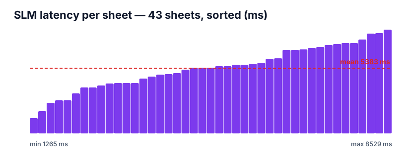
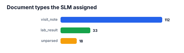
Per-sheet SLM latency ran a mean of 5,383 ms (min 1,265, max 8,529) — the spread tracks how much text was on each page. The model assigned every sheet a document type:
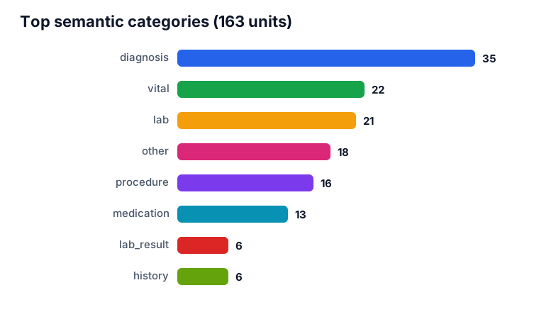
4. Semantic units. Across the 43 sheets the SLM emitted 163 semantic units — self-contained health facts, each tagged with a category. Diagnoses, vitals, and labs dominate, which is what a primary-care history should look like:
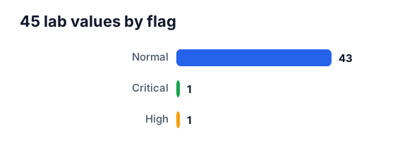
5. Track the labs carefully. Lab reports get a second, dedicated pass. Eleven sheets carried laboratory data; a lab-specific SLM prompt pulled every analyte as a structured row — test name, value, unit, reference range, and high/low/critical flag — yielding 45 lab values. The panel is exactly what you would expect from routine care: lipid panel, Hemoglobin A1c, a full CBC differential, a metabolic panel, urinalysis, and even a pure-tone audiometry result. Forty-two came back within reference range; the pass caught one high and one critical flag — precisely the two rows that most warrant attention and are easiest to miss in a stack of faxes.
6. Store and connect. Every unit and lab value is embedded to a 768-dimension vector by a local embedding service and written to pgvector — 208 vectors in two tables. Then the value that paper can never give you: a similarity search across sheets found 59 cross-document semantic bridges (23 of them near-identical, cosine > 0.90). Every one of the 43 sheets links to at least one other. A diagnosis on sheet 9 and its follow-up mention on sheet 25 are now one query apart, though they arrived in the stack sixteen pages away from each other.
The numbers
| Stage | Unit | Rate |
|---|---|---|
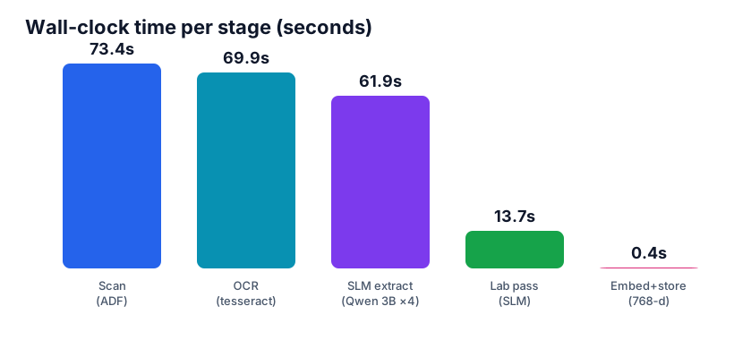
| Scan (ADF) | 43 sheets | 1.71 s/sheet |
| OCR (tesseract) | 43 sheets | 1.63 s/sheet |
| SLM understanding (Qwen 3B ×4) | 43 sheets | 5.38 s/sheet mean latency |
| Careful lab pass (SLM) | 11 sheets | 45 lab values, 13.7 s total |
| Embed + store (768-d) | 208 vectors | 52 ms bulk insert |
| Cross-sheet similarity | — | 59 semantic bridges |
End to end: the full run — first sheet on the glass to published story — took 12.3 minutes, a throughput of 13.3 semantic units per minute (16.9 vectors per minute, 3.5 sheets per minute). One person, one scanner, one consumer GPU, and no data-processing agreement with anyone — because no third party was involved.
Why local matters here
Health records are the canonical case where convenience and confidentiality pull in opposite directions. The usual cloud-LLM pipeline would have been faster per token, but it would have meant transmitting a named individual’s diagnoses and lab values to an external service. Running the understanding step on a 3B model on-prem removes that trade entirely: the model is good enough to classify documents and extract structured facts, small enough to run on a single local GPU, and private by construction. The cloud model orchestrating this write-up never saw a single lab value — it saw counts, timings, and category names, which is all a story needs.
Reproducibility
The pipeline is three small programs — a scan-and-split shell script, a parallel extraction script that calls the local SLM and embedding services, and a lab-specific pass — run against the same pgvector database that answers the queries. The identical pipeline serves any collection of scanned documents; point the SLM prompt at a different domain and it stops being about health at all. The interesting constraint was never the model size. It was keeping the entire loop on local hardware.